Labeled Dataset

The CSD model also supports labeled dimensions. In the following example, we present a mixed linear and labeled two-dimensional dataset representing the population of the country as a function of time. The dataset is obtained from The World Bank.

Import the csdmpy model and load the dataset.

import csdmpy as cp

filename = "https://www.ssnmr.org/sites/default/files/CSDM/labeled/population.csdf"
labeled_data = cp.load(filename)

The tuple of dimension and dependent variable objects from labeled_data instance are

x = labeled_data.dimensions
y = labeled_data.dependent_variables

Since one of the dimensions is a labeled dimension, let’s make use of the type attribute of the dimension instances to find out which dimension is labeled.

print(x[0].type)

linear

print(x[1].type)

labeled

Here, the second dimension is the labeled dimension with [1]

print(x[1].count)

263

labels, where the first five labels are

print(x[1].labels[:5])

['Aruba' 'Afghanistan' 'Angola' 'Albania' 'Andorra']

Note

For labeled dimensions, the coordinates attribute is an alias of the labels attribute.

print(x[1].coordinates[:5])

['Aruba' 'Afghanistan' 'Angola' 'Albania' 'Andorra']

The coordinates along the first dimension, viewed up to the first ten points, are

print(x[0].coordinates[:10])

[1960. 1961. 1962. 1963. 1964. 1965. 1966. 1967. 1968. 1969.] yr

Plotting the dataset

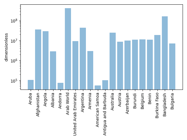
You may plot this dataset however you like. Here, we use a bar graph to represent the population of countries in the year 2017. The data corresponding to this year is a cross-section of the dependent variable at index 57 along the x[0] dimension.

print(x[0].coordinates[57])

2017.0 yr

To keep the plot simple, we only plot the first 20 country labels along the x[1] dimension.

import matplotlib.pyplot as plt
import numpy as np

x_data = x[1].coordinates[:20]
x_pos = np.arange(20)
y_data = y[0].components[0][:20, 57]

plt.bar(x_data, y_data, align="center", alpha=0.5)
plt.xticks(x_pos, x_data, rotation=90)
plt.ylabel(y[0].axis_label[0])
plt.yscale("log")
plt.title(y[0].name)
plt.tight_layout()
plt.show()

Footnotes

[1]

In the CSD model, the attribute count is only valid for the LinearDimension. In csdmpy, however, the count attribute is valid for all dimension objects and returns an integer with the number of grid points along the dimension.