
Getting started with csdmpy package
We have put together a set of guidelines for importing the csdmpy package and related methods and attributes. We encourage the users to follow these guidelines to promote consistency, amongst others. Import the package using
>>> import csdmpy as cp
To load a .csdf or a .csdfe file, use the load()
method of the csdmpy module. In the following example, we load a
sample test file.
>>> filename = "https://www.ssnmr.org/sites/default/files/CSDM/test/test01.csdf"
>>> testdata1 = cp.load(filename)
Here, testdata1 is an instance of the CSDM class.
At the root level, the CSDM object includes various useful optional
attributes that may contain additional information about the dataset. One such
useful attribute is the description key, which briefs
the end-users on the contents of the dataset. To access the value of this
attribute use,
>>> testdata1.description
'A simulated sine curve.'
Accessing dimensions and dependent variables of the dataset
An instance of the CSDM object may include multiple dimensions and
dependent variables. Collectively, the dimensions form a multi-dimensional grid
system, and the dependent variables populate this grid.
In csdmpy,
dimensions and dependent variables are structured as list object.
To access these lists, use the dimensions and
dependent_variables attribute of the CSDM object,
respectively. For example,
>>> x = testdata1.dimensions
>>> y = testdata1.dependent_variables
In this example, the dataset contains one dimension and one dependent variable.
You may access the instances of individual dimension and dependent variable by
using the proper indexing. For example, the dimension and dependent variable
at index 0 may be accessed using x[0] and y[0], respectively.
Every instance of the Dimension object has its own set of attributes
that further describe the respective dimension. For example, a Dimension object
may have an optional description
attribute,
>>> x[0].description
'A temporal dimension.'
Similarly, every instance of the DependentVariable object has its own set of
attributes. In this example, the
description
attribute from the dependent variable is
>>> y[0].description
'A response dependent variable.'
Coordinates along the dimension
Every dimension object contains a list of coordinates associated with every
grid index along the dimension. To access these coordinates, use
the coordinates attribute of the
respective Dimension instance. In this example, the coordinates are
>>> x[0].coordinates
<Quantity [0. , 0.1, 0.2, 0.3, 0.4, 0.5, 0.6, 0.7, 0.8, 0.9] s>
Note
x[0].coordinates returns a
Quantity
instance from the
Astropy package.
The csdmpy module utilizes the units library from
astropy.units module
to handle physical quantities. The numerical value and the
unit of the physical quantities are accessed through the Quantity
instance, using the value and the unit attributes, respectively.
Please refer to the astropy.units
documentation for details.
In the csdmpy module, the Quantity.value is a
Numpy array.
For instance, in the above example, the underlying Numpy array from the
coordinates attribute is accessed as
>>> x[0].coordinates.value
array([0. , 0.1, 0.2, 0.3, 0.4, 0.5, 0.6, 0.7, 0.8, 0.9])
Components of the dependent variable
Every dependent variable object has at least one component. The number of
components of the dependent variable is determined from the
quantity_type attribute
of the dependent variable object. For example, a scalar quantity has
one-component, while a vector quantity may have multiple components. To access
the components of the dependent variable, use the
components
attribute of the respective DependentVariable instance. For example,
>>> y[0].components
array([[ 0.0000000e+00,  5.8778524e-01,  9.5105654e-01,  9.5105654e-01,
         5.8778524e-01,  1.2246469e-16, -5.8778524e-01, -9.5105654e-01,
        -9.5105654e-01, -5.8778524e-01]], dtype=float32)
The components attribute
is a Numpy array. Note, the number of dimensions of this array is \(d+1\),
where \(d\) is the number of Dimension objects from the
dimensions attribute. The additional dimension in the
Numpy array corresponds to the number of components of the dependent variable.
For instance, in this example, there is a single dimension, i.e., \(d=1\)
and, therefore, the value of the
components
attribute holds a two-dimensional Numpy array of shape
>>> y[0].components.shape
(1, 10)
where the first element of the shape tuple, 1, is the number of
components of the dependent variable and the second element, 10, is the
number of points along the dimension, i.e., x[0].coordinates.
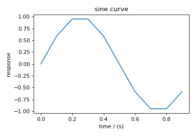
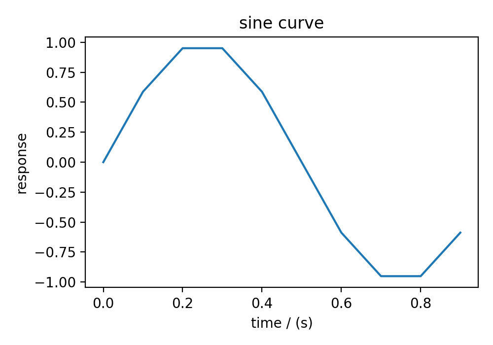
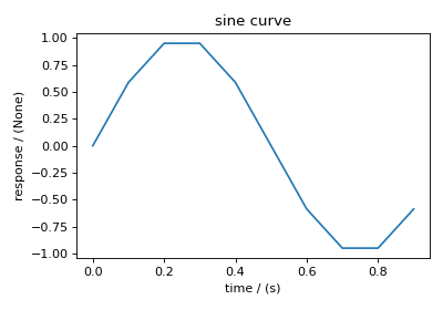
Plotting the dataset
It is always helpful to represent a scientific dataset with visual aids such as a plot or a figure instead of columns of numbers. As such, throughout this documentation, we provide a figure or two for every example dataset. We make use of Python’s Matplotlib library for generating these figures. The users may, however, use their favorite plotting library.
The following snippet plots the dataset from this example. Here, the axis_label is an attribute of both Dimension and DependentVariable instances, and the name is an attribute of the DependentVariable instance.
>>> import matplotlib.pyplot as plt

>>> plt.figure(figsize=(5, 3.5))
>>> plt.plot(x[0].coordinates, y[0].components[0])
>>> plt.xlabel(x[0].axis_label)
>>> plt.ylabel(y[0].axis_label[0])
>>> plt.title(y[0].name)
>>> plt.tight_layout()
>>> plt.show()
(Source code, png, hires.png, pdf)
See also
CSDM, Dimension, DependentVariable, Quantity, numpy array, Matplotlib library