
Note
Go to the end to download the full example code.
Global Mean Sea Level rise dataset
The following dataset is the Global Mean Sea Level (GMSL) rise from the late 19th to the Early 21st Century [1]. The original dataset was downloaded as a CSV file and subsequently converted to the CSD model format.
Let’s import this file.
The variable filename is a string with the address to the .csdf file.
The load() method of the csdmpy module reads the
file and returns an instance of the CSDM class, in
this case, as a variable sea_level. For a quick preview of the data
structure, use the data_structure attribute of this
instance.
print(sea_level.data_structure)
{
  "csdm": {
    "version": "1.0",
    "read_only": true,
    "timestamp": "2019-05-21T13:43:00Z",
    "tags": [
      "Jason-2",
      "satellite altimetry",
      "mean sea level",
      "climate"
    ],
    "description": "Global Mean Sea Level (GMSL) rise from the late 19th to the Early 21st Century.",
    "dimensions": [
      {
        "type": "linear",
        "count": 1608,
        "increment": "0.08333333333 yr",
        "coordinates_offset": "1880.0416666667 yr",
        "quantity_name": "time",
        "reciprocal": {
          "quantity_name": "frequency"
        }
      }
    ],
    "dependent_variables": [
      {
        "type": "internal",
        "name": "Global Mean Sea Level",
        "unit": "mm",
        "quantity_name": "length",
        "numeric_type": "float32",
        "quantity_type": "scalar",
        "component_labels": [
          "GMSL"
        ],
        "components": [
          [
            "-183.0, -171.125, ..., 59.6875, 58.5"
          ]
        ]
      }
    ]
  }
}
Warning
The serialized string from the data_structure
attribute is not the same as the JSON serialization on the file.
This attribute is only intended for a quick preview of the data
structure and avoids displaying large datasets. Do not use
the value of this attribute to save the data to the file. Instead, use the
save() method of the CSDM
class.
The tuple of the dimensions and dependent variables, from this example, are
respectively. The coordinates along the dimension and the component of the dependent variable are
print(x[0].coordinates)
[1880.04166667 1880.125      1880.20833333 ... 2013.79166666 2013.87499999
 2013.95833333] yr
and
print(y[0].components[0])
[-183. -171.125 -164.25 ... 66.375 59.6875 58.5 ]
respectively.
Plotting the data
Note
The following code is only for illustrative purposes. The users may use any plotting library to visualize their datasets.
import matplotlib.pyplot as plt

plt.figure(figsize=(5, 3.5))
ax = plt.subplot(projection="csdm")

# csdmpy is compatible with matplotlib function. Use the csdm object as the argument
# of the matplotlib function.
ax.plot(sea_level)
plt.tight_layout()
plt.show()
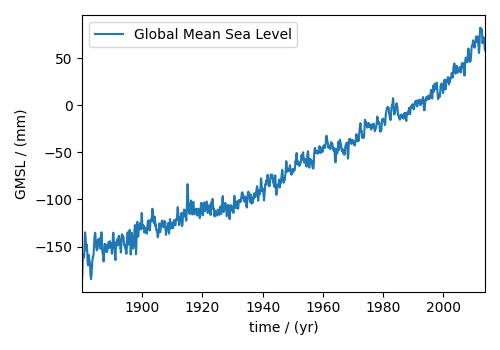
The following is a quick description of the above code. Within the code, we
make use of the csdm instance’s attributes in addition to the matplotlib
functions. The first line is an import call for the matplotlib functions.
The following line generates a plot of the coordinates along the
dimension verse the component of the dependent variable.
The next line sets the x-range. For labeling the axes,
use the axis_label attribute
of both dimension and dependent variable instances. For the figure title,
use the name attribute
of the dependent variable instance. The next statement adds the grid lines.
For additional information, refer to Matplotlib
documentation.
See also
Citation
Total running time of the script: (0 minutes 0.467 seconds)