
Note
Go to the end to download the full example code.
Nuclear Magnetic Resonance (NMR) dataset
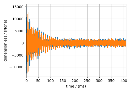
The following dataset is a \(^{13}\mathrm{C}\) time-domain NMR Bloch decay signal of ethanol. Let’s load this data file and take a quick look at its data structure. We follow the steps described in the previous example.
import matplotlib.pyplot as plt

import csdmpy as cp

domain = "https://www.ssnmr.org/sites/default/files/CSDM"
filename = f"{domain}/NMR/blochDecay/blochDecay.csdf"
NMR_data = cp.load(filename)
print(NMR_data.data_structure)
{
  "csdm": {
    "version": "1.0",
    "read_only": true,
    "timestamp": "2016-03-12T16:41:00Z",
    "geographic_coordinate": {
      "altitude": "238.9719543457031 m",
      "longitude": "-83.05154573892345 °",
      "latitude": "39.97968794964322 °"
    },
    "tags": [
      "13C",
      "NMR",
      "spectrum",
      "ethanol"
    ],
    "description": "A time domain NMR 13C Bloch decay signal of ethanol.",
    "dimensions": [
      {
        "type": "linear",
        "count": 4096,
        "increment": "0.1 ms",
        "coordinates_offset": "-0.3 ms",
        "quantity_name": "time",
        "reciprocal": {
          "coordinates_offset": "-3005.363 Hz",
          "origin_offset": "75426328.86 Hz",
          "quantity_name": "frequency",
          "label": "13C frequency shift"
        }
      }
    ],
    "dependent_variables": [
      {
        "type": "internal",
        "numeric_type": "complex128",
        "quantity_type": "scalar",
        "components": [
          [
            "(-8899.40625-1276.7734375j), (-4606.88037109375-742.4124755859375j), ..., (37.548492431640625+20.156890869140625j), (-193.9228515625-67.06524658203125j)"
          ]
        ]
      }
    ]
  }
}
This particular example illustrates two additional attributes of the CSD model,
namely, the geographic_coordinate and
tags. The geographic_coordinate described the
location where the CSDM file was last serialized. You may access this
attribute through,
{'altitude': '238.9719543457031 m', 'longitude': '-83.05154573892345 °', 'latitude': '39.97968794964322 °'}
The tags attribute is a list of keywords that best describe the dataset. The tags attribute is accessed through,
print(NMR_data.tags)
['13C', 'NMR', 'spectrum', 'ethanol']
You may add additional tags, if so desired, using the append method of python’s list class, for example,
NMR_data.tags.append("Bloch decay")
print(NMR_data.tags)
['13C', 'NMR', 'spectrum', 'ethanol', 'Bloch decay']
The coordinates along the dimension are
x = NMR_data.dimensions
x0 = x[0].coordinates
print(x0)
[-3.000e-01 -2.000e-01 -1.000e-01 ... 4.090e+02 4.091e+02 4.092e+02] ms
Unlike the previous example, the data structure of an NMR measurement is
a complex-valued dependent variable. The numeric type of the components from
a dependent variable is accessed through the
numeric_type attribute.
y = NMR_data.dependent_variables
print(y[0].numeric_type)
complex128
Visualizing the dataset
In the previous example, we illustrated a matplotlib script for plotting 1D data.
Here, we use the csdmpy plot() method, which is a supplementary method
for plotting 1D and 2D datasets only.
plt.figure(figsize=(5, 3.5))
ax = plt.subplot(projection="csdm")
ax.plot(NMR_data.real, label="real")
ax.plot(NMR_data.imag, label="imag")
plt.grid()
plt.tight_layout()
plt.show()
Reciprocal dimension object
When observing the dimension instance of NMR_data,
print(x[0].data_structure)
{
  "type": "linear",
  "count": 4096,
  "increment": "0.1 ms",
  "coordinates_offset": "-0.3 ms",
  "quantity_name": "time",
  "reciprocal": {
    "coordinates_offset": "-3005.363 Hz",
    "origin_offset": "75426328.86 Hz",
    "quantity_name": "frequency",
    "label": "13C frequency shift"
  }
}
notice, the reciprocal keyword. The reciprocal
attribute is useful for datasets that frequently transform to a reciprocal domain,
such as the NMR dataset. The value of the reciprocal attribute is the reciprocal
object, which contains metadata for describing the reciprocal coordinates, such as
the coordinates_offset, origin_offset of the reciprocal dimension.
You may perform a fourier transform to visualize the NMR spectrum. Use the
fft() method on the csdm object NMR_data as follows
By default, the unit associated with a dimension after FFT is the reciprocal of the unit associated with the dimension before FFT. In this case, the dimension unit after FFT is Hz. NMR datasets are often visualized as a dimension frequency scale. To convert the dimension’s unit to ppm use,
fft_NMR_data.dimensions[0].to("ppm", "nmr_frequency_ratio")

# plot of the frequency domain data after FFT.
fig, ax = plt.subplots(1, 2, figsize=(8, 3), subplot_kw={"projection": "csdm"})
ax[0].plot(fft_NMR_data.real, label="real")
plt.grid()
ax[1].plot(fft_NMR_data.imag, label="imag")
plt.grid()
plt.tight_layout()
plt.show()
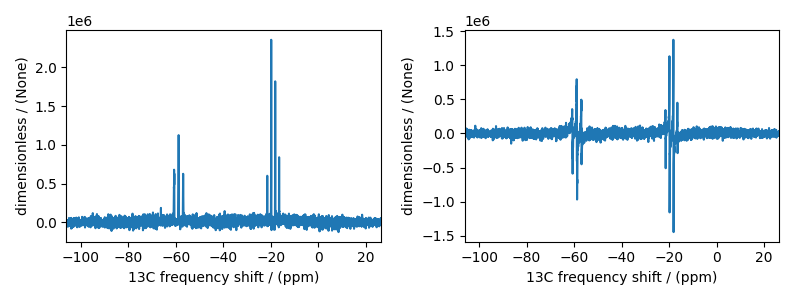
In the above plot, the plot metadata is taken from the reciprocal object such as the x-axis label.
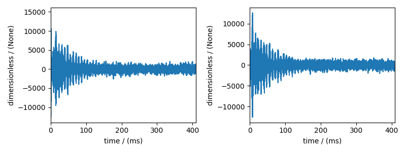
To return to time domain signal, once again use the fft() method
on the fft_NMR_data object. We use the CSDM object’s
complex_fft attribute to determine the FFT ot iFFT operation.
NMR_data_2 = fft_NMR_data.fft()

# plot of the frequency domain data.
fig, ax = plt.subplots(1, 2, figsize=(8, 3), subplot_kw={"projection": "csdm"})
ax[0].plot(NMR_data_2.real, label="real")
plt.grid()
ax[1].plot(NMR_data_2.imag, label="imag")
plt.grid()
plt.tight_layout()
plt.show()
Total running time of the script: (0 minutes 0.476 seconds)