
Note
Go to the end to download the full example code.
Sparse along two dimensions, 2D{1,1} dataset
The following is an example [1] of a 2D{1,1} sparse dataset with two-dimensions, \(d=2\), and two, \(p=2\), sparse single-component dependent-variables, where the component is sparsely sampled along two dimensions. The following is an example of a hypercomplex acquisition of the NMR dataset.
Let’s import the CSD model data-file and look at its data structure.
There are two linear dimensions and two single-component sparse dependent variables. The tuple of the dimension and the dependent variable instances are
The coordinates, viewed only for the first ten coordinates, are
print(x[0].coordinates[:10])
[ 0. 192. 384. 576. 768. 960. 1152. 1344. 1536. 1728.] us
print(x[1].coordinates[:10])
[ 0. 192. 384. 576. 768. 960. 1152. 1344. 1536. 1728.] us
Converting the coordinates to ms.
x[0].to("ms")
x[1].to("ms")
Visualize the dataset
import matplotlib.pyplot as plt
# split the CSDM object with two dependent variables into two CSDM objects with single
# dependent variables.
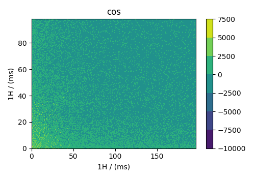
cos, sin = sparse_2d.split()
# cosine data
plt.figure(figsize=(5, 3.5))
ax = plt.subplot(projection="csdm")
cb = ax.contourf(cos.real)
plt.colorbar(cb, ax=ax)
plt.tight_layout()
plt.show()
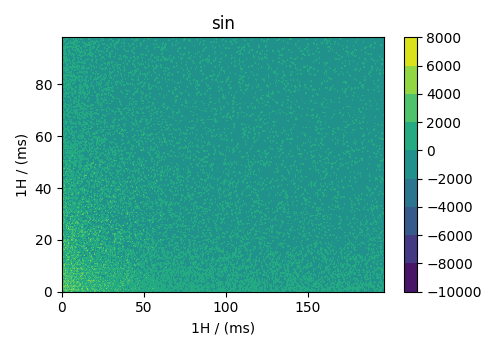
# sine data
plt.figure(figsize=(5, 3.5))
ax = plt.subplot(projection="csdm")
cb = ax.contourf(sin.real)
plt.colorbar(cb, ax=ax)
plt.tight_layout()
plt.show()
Citation
Total running time of the script: (0 minutes 0.686 seconds)