Vector, 2D{2} dataset

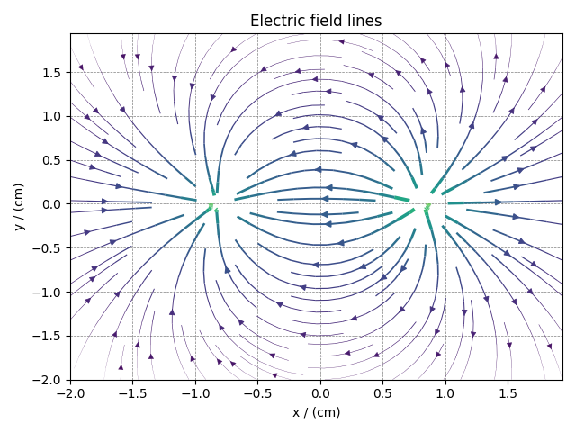
The 2D{2} datasets are two-dimensional, \(d=2\), with one two-component dependent variable, \(p=2\). The following is an example of a simulated electric field vector dataset of a dipole as a function of two linearly sampled spatial dimensions.

import csdmpy as cp

domain = "https://www.ssnmr.org/sites/default/files/CSDM"
filename = f"{domain}/vector/electric_field/electric_field_base64.csdf"

vector_data = cp.load(filename)
print(vector_data.data_structure)

{
  "csdm": {
    "version": "1.0",
    "read_only": true,
    "timestamp": "2014-09-30T11:16:33Z",
    "description": "A simulated electric field dataset from an electric dipole.",
    "dimensions": [
      {
        "type": "linear",
        "count": 64,
        "increment": "0.0625 cm",
        "coordinates_offset": "-2.0 cm",
        "quantity_name": "length",
        "label": "x",
        "reciprocal": {
          "quantity_name": "wavenumber"
        }
      },
      {
        "type": "linear",
        "count": 64,
        "increment": "0.0625 cm",
        "coordinates_offset": "-2.0 cm",
        "quantity_name": "length",
        "label": "y",
        "reciprocal": {
          "quantity_name": "wavenumber"
        }
      }
    ],
    "dependent_variables": [
      {
        "type": "internal",
        "name": "Electric field lines",
        "unit": "C^-1 * N",
        "quantity_name": "electric field strength",
        "numeric_type": "float32",
        "quantity_type": "vector_2",
        "components": [
          [
            "3.7466873e-07, 3.3365018e-07, ..., 3.5343004e-07, 4.0100363e-07"
          ],
          [
            "1.6129676e-06, 1.6765767e-06, ..., 1.846712e-06, 1.7754871e-06"
          ]
        ]
      }
    ]
  }
}

The tuple of the dimension and dependent variable instances from this example are

x = vector_data.dimensions
y = vector_data.dependent_variables

with the respective coordinates (viewed only up to five values), as

print(x[0].coordinates[:5])

[-2.     -1.9375 -1.875  -1.8125 -1.75  ] cm

print(x[1].coordinates[:5])

[-2.     -1.9375 -1.875  -1.8125 -1.75  ] cm

The components of the dependent variable are vector components as seen from the quantity_type attribute of the corresponding dependent variable instance.

print(y[0].quantity_type)

vector_2

Visualizing the dataset

Let’s visualize the vector data using the streamplot method from the matplotlib package. Before we could visualize, however, there is an initial processing step. We use the Numpy library for processing.

import numpy as np

X, Y = np.meshgrid(x[0].coordinates, x[1].coordinates)  # (x, y) coordinate pairs
U, V = y[0].components[0], y[0].components[1]  # U and V are the components
R = np.sqrt(U**2 + V**2)  # The magnitude of the vector
R /= R.min()  # Scaled magnitude of the vector
Rlog = np.log10(R)  # Scaled magnitude of the vector on a log scale

In the above steps, we calculate the X-Y grid points along with a scaled magnitude of the vector dataset. The magnitude is scaled such that the minimum value is one. Next, calculate the log of the scaled magnitude to visualize the intensity on a logarithmic scale.

And now, the streamplot vector plot

import matplotlib.pyplot as plt

plt.streamplot(
    X.value, Y.value, U, V, density=1, linewidth=Rlog, color=Rlog, cmap="viridis"
)

plt.xlim([x[0].coordinates[0].value, x[0].coordinates[-1].value])
plt.ylim([x[1].coordinates[0].value, x[1].coordinates[-1].value])

# Set axes labels and figure title.
plt.xlabel(x[0].axis_label)
plt.ylabel(x[1].axis_label)
plt.title(y[0].name)

# Set grid lines.
plt.grid(color="gray", linestyle="--", linewidth=0.5)

plt.tight_layout()
plt.show()