
Note
Go to the end to download the full example code.
Diffusion tensor MRI, 3D{6} dataset
The following is an example of a 3D{6} diffusion tensor MRI dataset with three spatial dimensions, \(d=3\), and one, \(p=1\), dependent-variable with six components. For illustration, we have reduced the size of the dataset. The complete diffusion tensor MRI dataset, in the CSDM format, is available online. The original dataset [1] is also available.
Let’s import the CSDM data-file and look at its data structure.
There are three linear dimensions in this dataset, corresponding to the x, y, and z spatial dimensions,
x = diff_mri.dimensions
print(x[0].label, x[1].label, x[2].label)
x y z
and one six-component dependent variables holding the diffusion tensor components. Because the diffusion tensor is a symmetric second-rank tensor, we only need six tensor components. The components of the tensor are ordered as
y = diff_mri.dependent_variables
print(y[0].component_labels)
['dxx', 'dxy', 'dxz', 'dyy', 'dyz', 'dzz']
The symmetric matrix information is also found with the
quantity_type attribute,
print(y[0].quantity_type)
symmetric_matrix_3
which implies a 3x3 symmetric matrix.
Visualize the dataset
In the following, we visualize the isotropic diffusion coefficient, that is, the average of the \(d_{xx}\), \(d_{yy}\), and \(d_{zz}\) tensor components. Since it’s a three-dimensional dataset, we’ll visualize the projections onto the three dimensions.
# the isotropic diffusion coefficient.
# component at index 0 = dxx
# component at index 3 = dyy
# component at index 5 = dzz
isotropic_diffusion = (y[0].components[0] + y[0].components[3] + y[0].components[5]) / 3
In the following, we use certain features of the csdmpy module. Please refer to Generating CSDM objects for further details.
# Create a new csdm object from the isotropic diffusion coefficient array.
new_csdm = cp.as_csdm(isotropic_diffusion, quantity_type="scalar")

# Add the dimensions from `diff_mri` object to the `new_csdm` object.
for i, dim in enumerate(x):
    new_csdm.dimensions[i] = dim
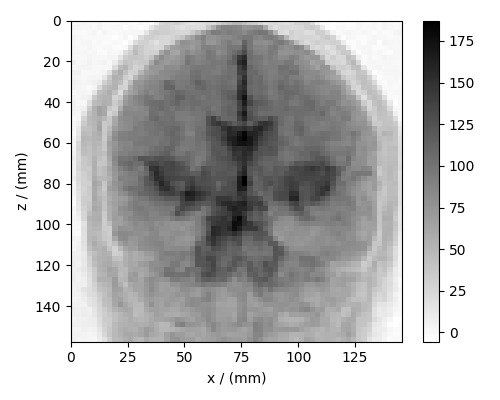
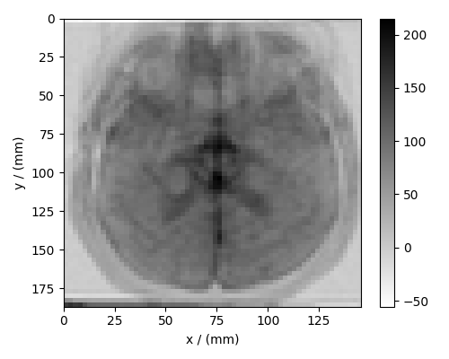
Now, we can plot the projections of the isotropic diffusion coefficients along the respective dimensions as
import matplotlib.pyplot as plt

# projection along the x-axis.
plt.figure(figsize=(5, 4))
ax = plt.subplot(projection="csdm")
cb = ax.imshow(new_csdm.sum(axis=0), cmap="gray_r", origin="upper", aspect="auto")
plt.colorbar(cb, ax=ax)
plt.tight_layout()
plt.show()
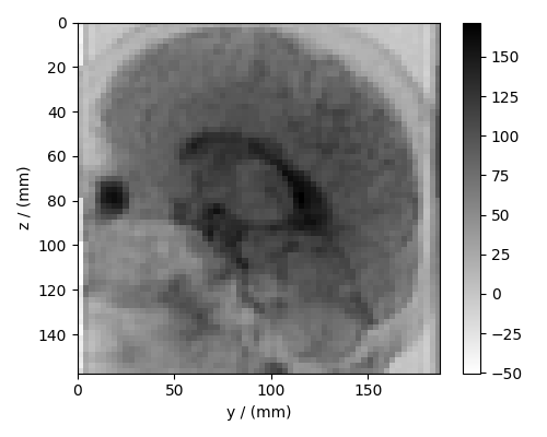
# projection along the y-axis.
plt.figure(figsize=(5, 4))
ax = plt.subplot(projection="csdm")
cb = ax.imshow(new_csdm.sum(axis=1), cmap="gray_r", origin="upper", aspect="auto")
plt.colorbar(cb, ax=ax)
plt.tight_layout()
plt.show()
# projection along the z-axis.
plt.figure(figsize=(5, 4))
ax = plt.subplot(projection="csdm")
cb = ax.imshow(new_csdm.sum(axis=2), cmap="gray_r", origin="upper", aspect="auto")
plt.colorbar(cb, ax=ax)
plt.tight_layout()
plt.show()
Citation
Total running time of the script: (0 minutes 0.431 seconds)