Linear and Monotonic dimensions

In the following example, we illustrate how one can covert a Numpy array into a CSDM object. Start by importing the Numpy and csdmpy libraries.

import matplotlib.pyplot as plt
import numpy as np

import csdmpy as cp

Let’s generate a 2D NumPy array of random numbers as our dataset.

data = np.random.rand(8192).reshape(32, 256)

To convert this array into a csdm object, use the as_csdm() method,

data_csdm = cp.as_csdm(data)
print(data_csdm.dimensions)

Out:

[LinearDimension(count=256, increment=1.0),
LinearDimension(count=32, increment=1.0)]

This generates a 2D{1} dataset, that is, a two-dimensional dataset with a single one-component dependent variable. The two dimensions are, by default, set as the LinearDimensions of the unit interval.

You may set the proper dimensions by generating the appropriate Dimension objects and replacing the default dimensions in the data_csdm object.

d0 = cp.LinearDimension(
    count=256, increment="15.23 µs", coordinates_offset="-1.95 ms", label="t1"
)

Here, d0 is a LinearDimension with 256 points and 15.23 µs increment. You may similarly set the second dimension as a LinearDimension, however, in this example, let’s set it as a MonotonicDimension.

array = 10 ** (np.arange(32) / 8)
d1 = cp.as_dimension(array, unit="µs", label="t2")

The variable array is a NumPy array that is uniformly sampled on a log scale. To convert this array into a Dimension object, we use the as_dimension() method.

Now, replace the dimension objects in data_csdm with the new ones.

data_csdm.dimensions[0] = d0
data_csdm.dimensions[1] = d1

print(data_csdm.dimensions)

Out:

[LinearDimension(count=256, increment=15.23 µs, coordinates_offset=-1.95 ms, quantity_name=time, label=t1, reciprocal={'quantity_name': 'frequency'}),
MonotonicDimension(coordinates=[1.00000000e+00 1.33352143e+00 1.77827941e+00 2.37137371e+00
 3.16227766e+00 4.21696503e+00 5.62341325e+00 7.49894209e+00
 1.00000000e+01 1.33352143e+01 1.77827941e+01 2.37137371e+01
 3.16227766e+01 4.21696503e+01 5.62341325e+01 7.49894209e+01
 1.00000000e+02 1.33352143e+02 1.77827941e+02 2.37137371e+02
 3.16227766e+02 4.21696503e+02 5.62341325e+02 7.49894209e+02
 1.00000000e+03 1.33352143e+03 1.77827941e+03 2.37137371e+03
 3.16227766e+03 4.21696503e+03 5.62341325e+03 7.49894209e+03] us, quantity_name=time, label=t2, reciprocal={'quantity_name': 'frequency'})]

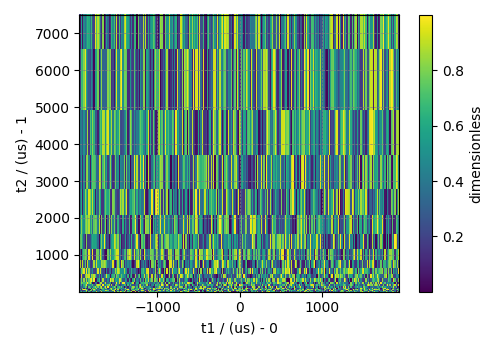
Plot of the dataset.

plt.figure(figsize=(5, 3.5))
cp.plot(data_csdm)
plt.tight_layout()
plt.show()

To serialize the file, use the save method.

data_csdm.save("filename.csdf")