
Note
Click here to download the full example code
Image, 2D{3} datasets
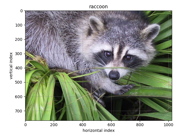
The 2D{3} dataset is two dimensional, \(d=2\), with a single three-component dependent variable, \(p=3\). A common example from this subset is perhaps the RGB image dataset. An RGB image dataset has two spatial dimensions and one dependent variable with three components corresponding to the red, green, and blue color intensities.
The following is an example of an RGB image dataset.
import csdmpy as cp

filename = "https://osu.box.com/shared/static/vdxdaitsa9dq45x8nk7l7h25qrw2baxt.csdf"
ImageData = cp.load(filename)
print(ImageData.data_structure)
Out:
{
  "csdm": {
    "version": "1.0",
    "read_only": true,
    "timestamp": "2016-03-12T16:41:00Z",
    "tags": [
      "racoon",
      "image",
      "Judy Weggelaar"
    ],
    "description": "An RBG image of a raccoon face.",
    "dimensions": [
      {
        "type": "linear",
        "count": 1024,
        "increment": "1.0",
        "label": "horizontal index"
      },
      {
        "type": "linear",
        "count": 768,
        "increment": "1.0",
        "label": "vertical index"
      }
    ],
    "dependent_variables": [
      {
        "type": "internal",
        "name": "raccoon",
        "numeric_type": "uint8",
        "quantity_type": "pixel_3",
        "component_labels": [
          "red",
          "green",
          "blue"
        ],
        "components": [
          [
            "121, 138, ..., 119, 118"
          ],
          [
            "112, 129, ..., 155, 154"
          ],
          [
            "131, 148, ..., 93, 92"
          ]
        ]
      }
    ]
  }
}
The tuple of the dimension and dependent variable instances from
ImageData instance are
respectively. There are two dimensions, and the coordinates along each dimension are
print("x0 =", x[0].coordinates[:10])
Out:
x0 = [0. 1. 2. 3. 4. 5. 6. 7. 8. 9.]
print("x1 =", x[1].coordinates[:10])
Out:
x1 = [0. 1. 2. 3. 4. 5. 6. 7. 8. 9.]
respectively, where only first ten coordinates along each dimension is displayed.
The dependent variable is the image data, as also seen from the
quantity_type attribute
of the corresponding DependentVariable instance.
print(y[0].quantity_type)
Out:
pixel_3
From the value pixel_3, pixel indicates a pixel data, while 3 indicates the number of pixel components.
As usual, the components of the dependent variable are accessed through
the components attribute.
To access the individual components, use the appropriate array indexing.
For example,
print(y[0].components[0])
Out:
[[121 138 153 ... 119 131 139]
 [ 89 110 130 ... 118 134 146]
 [ 73  94 115 ... 117 133 144]
 ...
 [ 87  94 107 ... 120 119 119]
 [ 85  95 112 ... 121 120 120]
 [ 85  97 111 ... 120 119 118]]
will return an array with the first component of all data values. In this case,
the components correspond to the red color intensity, also indicated by the
corresponding component label. The label corresponding to
the component array is accessed through the
component_labels
attribute with appropriate indexing, that is
print(y[0].component_labels[0])
Out:
red
To avoid displaying larger output, as an example, we print the shape of each component array (using Numpy array’s shape attribute) for the three components along with their respective labels.
print(y[0].component_labels[0], y[0].components[0].shape)
Out:
red (768, 1024)
print(y[0].component_labels[1], y[0].components[1].shape)
Out:
green (768, 1024)
print(y[0].component_labels[2], y[0].components[2].shape)
Out:
blue (768, 1024)
The shape (768, 1024) corresponds to the number of points from the each dimension instances.
Note
In this example, since there is only one dependent variable, the index
of y is set to zero, which is y[0]. The indices for the
components and the
component_labels,
on the other hand, spans through the number of components.
Now, to visualize the dataset as an RGB image,
import matplotlib.pyplot as plt

ax = plt.subplot(projection="csdm")
ax.imshow(ImageData, origin="upper")
plt.tight_layout()

plt.show()
Total running time of the script: ( 0 minutes 1.551 seconds)