
Note
Click here to download the full example code
Nuclear Magnetic Resonance (NMR) dataset
The following dataset is a \(^{13}\mathrm{C}\) time-domain NMR Bloch decay signal of ethanol. Let’s load this data file and take a quick look at its data structure. We follow the steps described in the previous example.
import matplotlib.pyplot as plt

import csdmpy as cp

filename = "https://osu.box.com/shared/static/2e4fqm8n8bh4i5wgrinbwcavafa8x7y1.csdf"
NMR_data = cp.load(filename)
print(NMR_data.data_structure)
Out:
{
  "csdm": {
    "version": "1.0",
    "read_only": true,
    "timestamp": "2016-03-12T16:41:00Z",
    "geographic_coordinate": {
      "altitude": "238.9719543457031 m",
      "longitude": "-83.05154573892345 °",
      "latitude": "39.97968794964322 °"
    },
    "tags": [
      "13C",
      "NMR",
      "spectrum",
      "ethanol"
    ],
    "description": "A time domain NMR 13C Bloch decay signal of ethanol.",
    "dimensions": [
      {
        "type": "linear",
        "count": 4096,
        "increment": "0.1 ms",
        "coordinates_offset": "-0.3 ms",
        "quantity_name": "time",
        "reciprocal": {
          "coordinates_offset": "-3005.363 Hz",
          "origin_offset": "75426328.86 Hz",
          "quantity_name": "frequency",
          "label": "13C frequency shift"
        }
      }
    ],
    "dependent_variables": [
      {
        "type": "internal",
        "numeric_type": "complex128",
        "quantity_type": "scalar",
        "components": [
          [
            "(-8899.40625-1276.7734375j), (-4606.88037109375-742.4124755859375j), ..., (37.548492431640625+20.156890869140625j), (-193.9228515625-67.06524658203125j)"
          ]
        ]
      }
    ]
  }
}
This particular example illustrates two additional attributes of the CSD model,
namely, the geographic_coordinate and
tags. The geographic_coordinate described the
location where the CSDM file was last serialized. You may access this
attribute through,
Out:
{'altitude': '238.9719543457031 m', 'longitude': '-83.05154573892345 °', 'latitude': '39.97968794964322 °'}
The tags attribute is a list of keywords that best describe the dataset. The tags attribute is accessed through,
Out:
['13C', 'NMR', 'spectrum', 'ethanol']
You may add additional tags, if so desired, using the append method of python’s list class, for example,
NMR_data.tags.append("Bloch decay")
NMR_data.tags
Out:
['13C', 'NMR', 'spectrum', 'ethanol', 'Bloch decay']
The coordinates along the dimension are
x = NMR_data.dimensions
x0 = x[0].coordinates
print(x0)
Out:
[-3.000e-01 -2.000e-01 -1.000e-01 ... 4.090e+02 4.091e+02 4.092e+02] ms
Unlike the previous example, the data structure of an NMR measurement is
a complex-valued dependent variable. The numeric type of the components from
a dependent variable is accessed through the
numeric_type attribute.
y = NMR_data.dependent_variables
print(y[0].numeric_type)
Out:
complex128
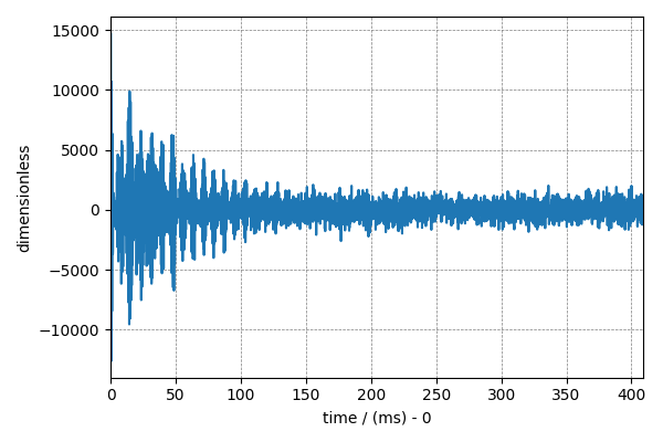
Visualizing the dataset
In the previous example, we illustrated a matplotlib script for plotting 1D data.
Here, we use the csdmpy plot() method, which is a supplementary method
for plotting 1D and 2D datasets only.
plt.figure(figsize=(6, 4))
cp.plot(NMR_data.real)
plt.tight_layout()
plt.show()
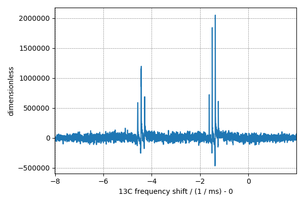
Reciprocal dimension object
When closely observing the dimension instance of NMR_data,
print(x[0].data_structure)
Out:
{
  "type": "linear",
  "count": 4096,
  "increment": "0.1 ms",
  "coordinates_offset": "-0.3 ms",
  "quantity_name": "time",
  "reciprocal": {
    "coordinates_offset": "-3005.363 Hz",
    "origin_offset": "75426328.86 Hz",
    "quantity_name": "frequency",
    "label": "13C frequency shift"
  }
}
notice, there is a reciprocal keyword. The
reciprocal attribute is useful for datasets
that frequently transform to a reciprocal domain, such as the NMR dataset.
The value of the reciprocal attribute is the reciprocal object, which contains metadata
for describing the reciprocal coordinates, such as the coordinates_offset,
origin_offset of the reciprocal dimension.
You may perform a fourier transform to visualize the NMR spectrum. Use the
fft() method on the csdm object NMR_data as follows
fft_NMR_data = NMR_data.fft()

# plot of the time domain data.
plt.figure(figsize=(6, 4))
cp.plot(fft_NMR_data.real)
plt.tight_layout()
plt.show()
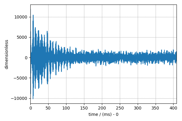
To return to time domain signal, use the fft() method on the
fft_NMR_data object,
NMR_data_2 = fft_NMR_data.fft()

# plot of the frequency domain data.
plt.figure(figsize=(6, 4))
cp.plot(NMR_data_2.real)
plt.tight_layout()
plt.show()
Total running time of the script: ( 0 minutes 1.473 seconds)